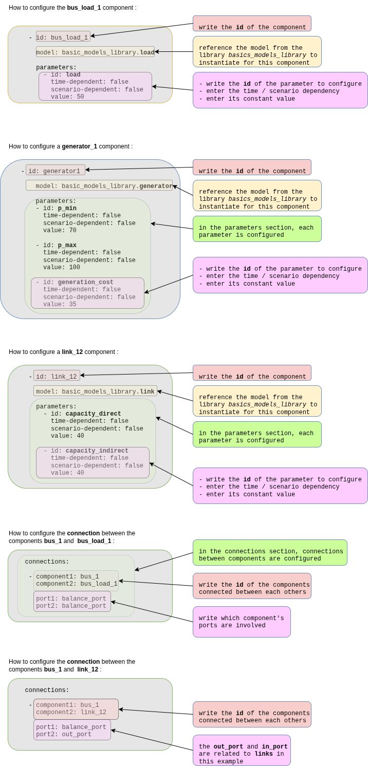
Quick-start example 1: three-bus adequacy system

Overview and problem description

This tutorial demonstrates adequacy modeling using a simplified three-bus meshed network over one single time-step. The example is intended to illustrate modeling concepts and should not be interpreted as a realistic system representation; however, it provides a foundation for developing more detailed and realistic models.

The study folder is on the GEMS Github repository.

Adequacy definition

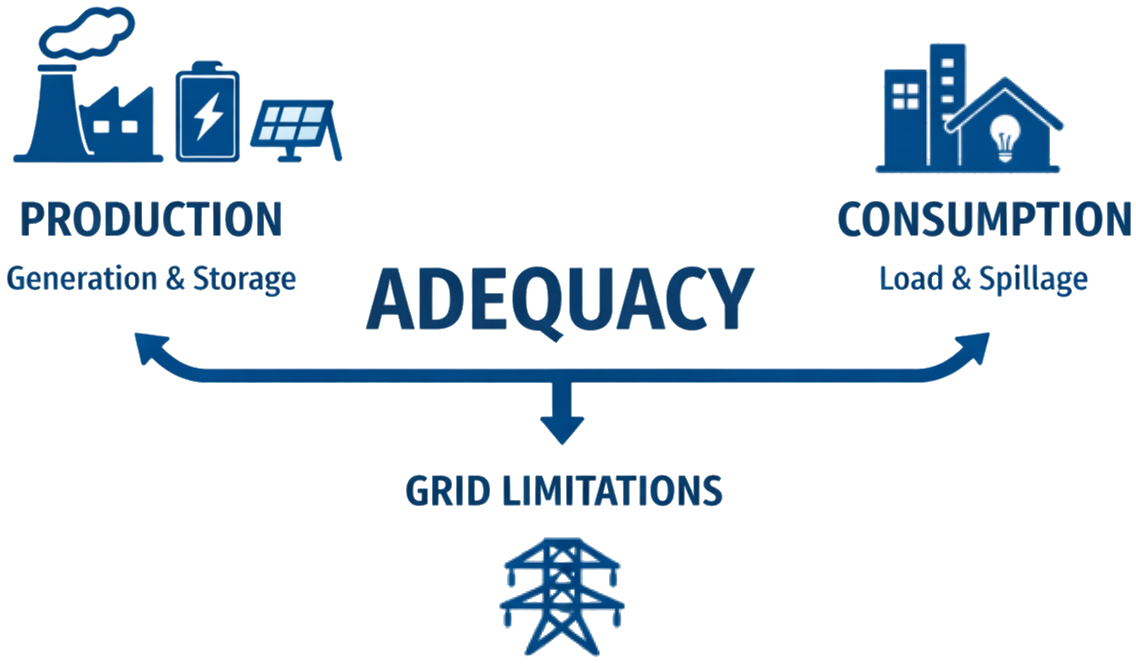
Adequacy is the ability of the electric grid to satisfy the end-user power demand at all times. The main challenge is to get the balance between the electric Production (generator, storage) and Consumption (load, spillage) while respecting the limitations of the grid.

Problem description

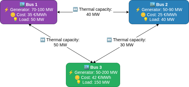
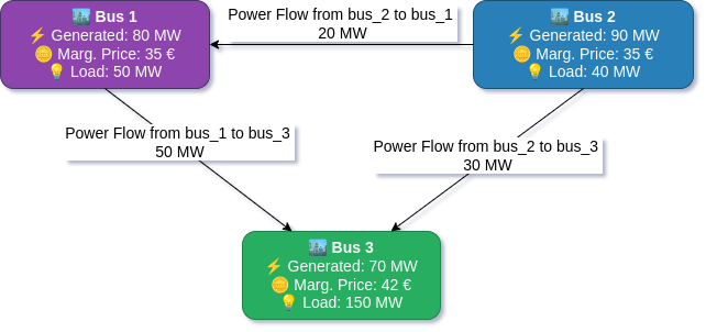
The following diagram represents the simulated system:

Problem description in detail

Time Horizon:

• This example considers a single one-hour time step.

Network Components:

• 3 Buses (Regions 1, 2, 3 forming a triangle)
• 3 Links (connecting each pair of regions)
• 3 Generators (different capacities and costs)
• 3 Loads (fixed demands)

In this example, the power flows on the links are constrained only by thermal capacities. Generation:

• Generator 1 (Bus 1): 70-100 MW capacity, 35 €/MWh cost
• Generator 2 (Bus 2): 50-90 MW capacity, 25 €/MWh cost
• Generator 3 (Bus 3): 50-200 MW capacity, 42 €/MWh cost

Demand:

• Bus 1: 50 MW
• Bus 2: 40 MW
• Bus 3: 150 MW
• Total Load: 240 MW

Transmission Capacities:

• Link 1-2: 40 MW (bidirectional)
• Link 2-3: 30 MW (bidirectional)
• Link 3-1: 50 MW (bidirectional)

Economic Parameters:

• Spillage cost: 1000 €/MWh (penalty for wasted energy)
• Unsupplied energy cost: 10000 €/MWh (high penalty for unmet demand)

The GEMS study

Files Structure

The following block represents the GEMS Framework study folder structure.

QSE_1_adequacy/
├── input/
│   ├──model-libraries/
│   │  └──  basic_models_library.yml 
│   ├── system.yml
│   └── data-series/
│       └──  ...
└── parameters.yml

The example study makes use of models provided by the GEMS library. For maintainability reasons, the library is stored separately in the repository and is not included directly in the example study. Consequently, users must copy the basic_models_library.yml file into the example study directory (QSE_1_adequacy/input/model-libraries/) prior to execution.

Since this example performs the simulation over a single time step, the data-series folder does not contain any time-series data.

Simulation options can be configured in the parameters.yml file. For more details on available simulation options, refer to the following link.

Relations between library and system files

The following diagram depicts the structural relationships between the library file and the system file:

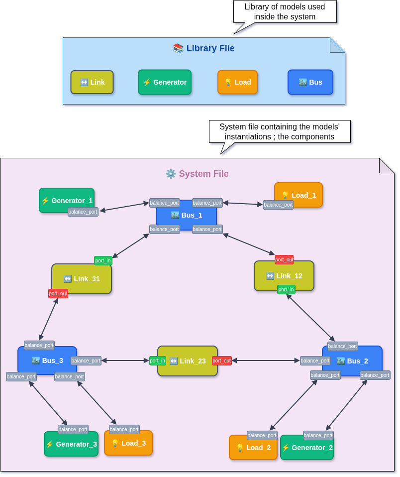
Library and System relations in details

The previous diagram represents the system.yml file, where users can instantiate components (such as buses, links, generators, etc.) and connect them via ports to form the optimization graph. It also illustrates the relationship between the library file and the system file for this adequacy example.

• Instantiation of components bus_1, bus_load_1, generator_1, and link_12 is shown, as well as the connections between bus_1 and bus_load_1, and between bus_1 and link_12.
• The complete system file can be found in this repository .

Running the GEMS study with Antares Modeler

⚠️ Warning
It's recommended to run this GEMS study with Antares Modeler or GemsPyIndeed, Antares Solver's hybrid mode manages GEMS objects, but there are some limitations regarding the temporal structure (8,760 timestep timeseries and weekly decomposition) related to the Legacy part of Antares Solver. For more information about the hybrid mode of Antares Solver, see the Hybrid Study section.

1. Download QSE_1_Adequacy
2. Copy basic_models_library.yml into the QSE_1_adequacy/input/model-libraries/
3. Get Antares Modeler installed through this tutorial
4. Locate bin folder
5. Open the terminal
6. Run these command lines :

# Windows
antares-modeler.exe <path-to-study>

# Linux
./antares-modeler <path-to-study>

Outputs

The results are available in the csv file QSE_1_Adequacy/output/simulation_table--YYYYMMDD-HHMM.csv

The simulation outputs contain the optimised value of optimisation problem variables, the status of all constraints and bounds, as well as user-defined extra output, as described on the following page.

The power flows between buses can be visualized as follows:

Outputs in details

By utilising the extra output feature, the marginal price is obtained as the dual value of the power balance constraint at each bus:

• bus_1: 35 €/MWh, based on the generation cost of generator_1.
• bus_2: 35 €/MWh, since generator_2 is operating at its maximum capacity. The next increment of 1 MWh is therefore produced by generator_1.
• bus_3: 42 €/MWh, based on the generation cost of generator_3.

The following graphs show the merit order of the generators and link flows:

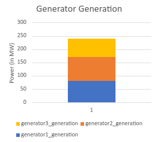
This graph shows the power output of each generator in the system, illustrating how the optimiser allocates generation based on cost and capacity constraints.

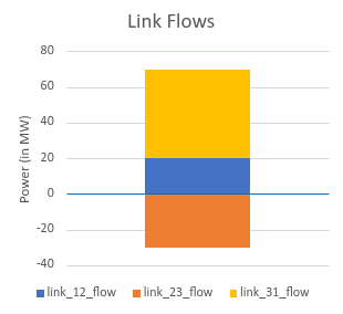
Above the blue abscissa axis, the flow represents import; below, it represents export.

Further in-depth explanations

Models Library

System of the Three-bus Adequacy example relies on models defined in the GEMS library file basic_models_library.yml. These models encode the decision variables, objective-function contributions, and constraints that collectively form the optimisation problem.

The complete mathematical formulation corresponding to this example — including decision variables, parameters, objective function, and constraints — is detailed in the following document: detailed mathematical formulation and expressions.

System file configuration

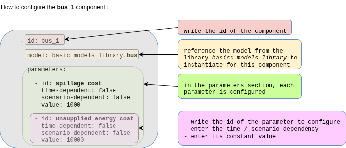
The description of an energy system is the combination of a model library and a graph of components (instanciation of models) described in the system file. For example, for the component bus_1, here is an extract of the system file :

Full system file description for the Three-bus system - Simple Adequacy Example

The following diagrams explains the structure of the system file for the Three-bus system - Simple Adequacy Example :